Computer vision · Structural health monitoring

Multi-defect concrete inspection with deep learning

I benchmarked YOLO-seg, U-Net and FPN models for crack and multi-defect segmentation, then tested them on real inspection photos from an industry partner. The field test showed where benchmark accuracy fails on site.

Context: MSc dissertation, Ulster University · industry partner Amphora Consulting (Belfast)
Period: 2025
My role: Sole researcher: data preparation, model training, field validation, practitioner survey

Code, model card & results: concrete-defect-detection-shm

U-Net (ResNet-50) crack segmentation on inspection images (dissertation Fig. 18).

0.807
Box mAP50: YOLOv8x-seg · Crack-Seg test; 0.630
mIoU (F1 0.775): U-Net ResNet-50 · validation split; 0.933
Field recall: YOLO11x-seg · 14 of 15 cracked images; 27 min
689 images, full pipeline + report: ≈2.38 s per image

Chapter 01

The engineering challenge

Visual inspection of reinforced concrete is slow, subjective and often done at height. In a survey I ran, the 21 professionals who responded said a medium-sized building typically takes 4–7 days to inspect.

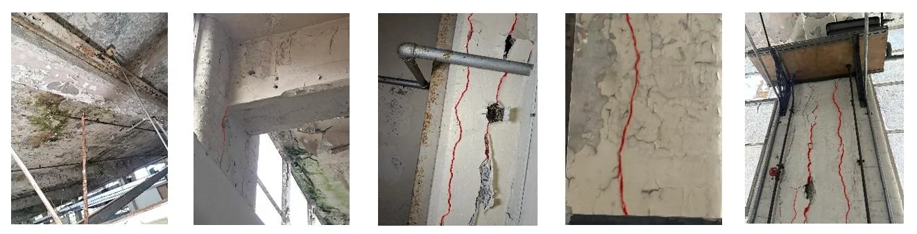
Published crack detectors report high benchmark scores. Site photos, however, are full of pipes, cables, coatings and shadows that look like cracks, so benchmark accuracy says little about field reliability.

Chapter 02

Input data

Crack-Seg benchmark

3,717 train · 112 val · 200 test images, 416 × 416

DACL10k

9,920 bridge-inspection images, 18 defect classes, polygon masks

Industry site photos

689 images from live projects in Belfast: pipes, coatings, shadows

Practitioner survey

21 professionals across the UK, KSA, UAE and Egypt

Three site photos with crack masks from three YOLO models side by side — External validation: the same site images through YOLO11x-seg, YOLO11n-seg and YOLOv8x-seg.

Chapter 03

The AI & engineering workflow

Stage 1 of 5

Data

Crack-Seg · DACL10k (9,920 images, 18 classes) · 689 industry site photos

What I did

Trained and compared three YOLO-seg variants (YOLOv8x, YOLO11x, YOLO11n) on the Crack-Seg dataset (3,717 / 112 / 200 images).
Trained a U-Net with a ResNet-50 encoder for pixel-accurate crack masks suitable for width and area measurement.
Extended to 18-class multi-defect segmentation on DACL10k with an FPN–EfficientNet-B4, using a Dice + weighted BCE loss, warm-up and cosine schedules, and mixed precision.
Ran an external validation on real site images from Amphora and classified every prediction by hand as TP/FP/TN/FN.
Designed and analysed a practitioner survey (UK, KSA, UAE, Egypt) to anchor the work in inspection practice.

PythonPyTorch 2.5Ultralytics YOLOsegmentation-models-pytorchAlbumentationsOpenCVRTX 4060 (8 GB)

Input → output

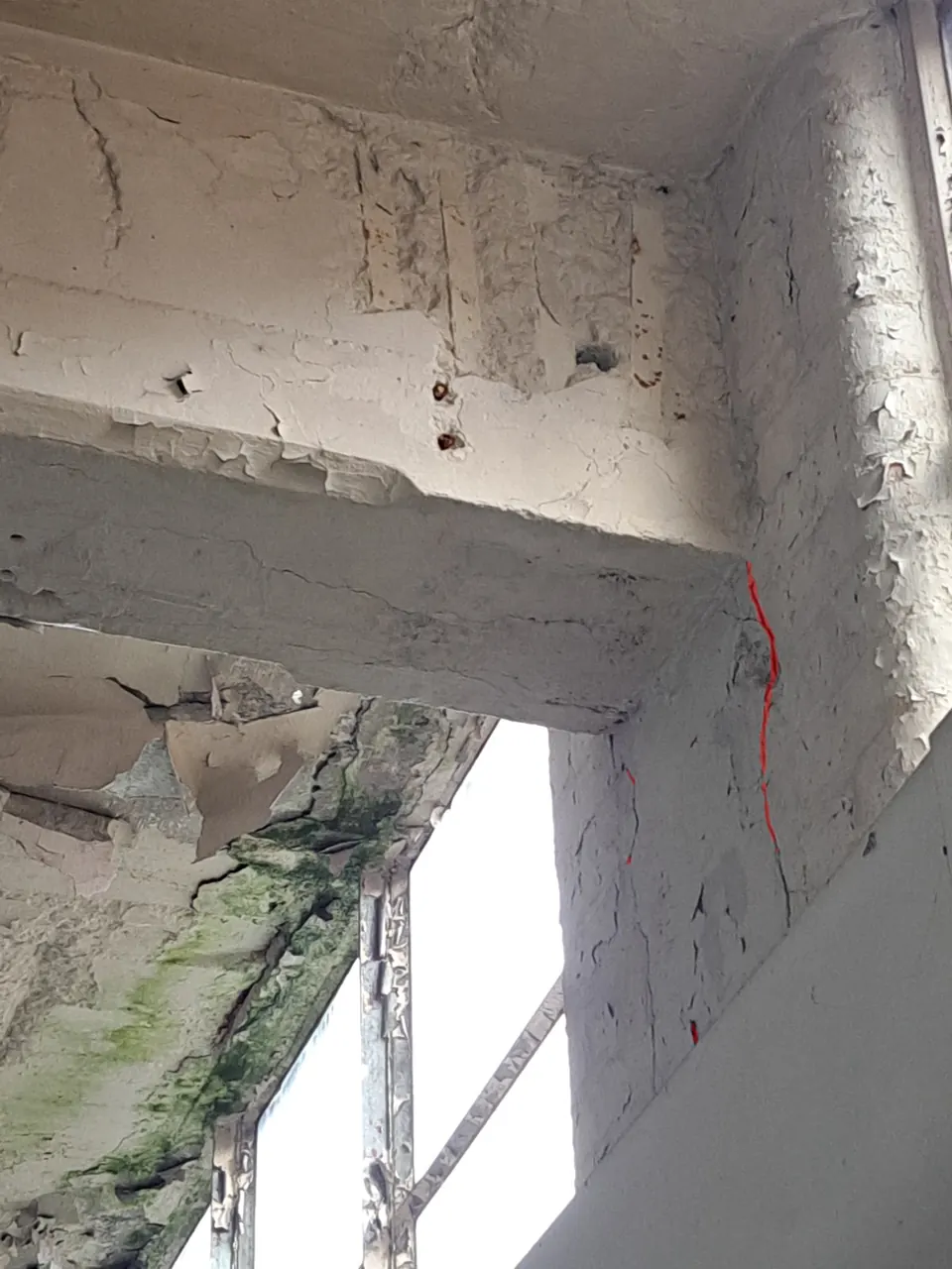
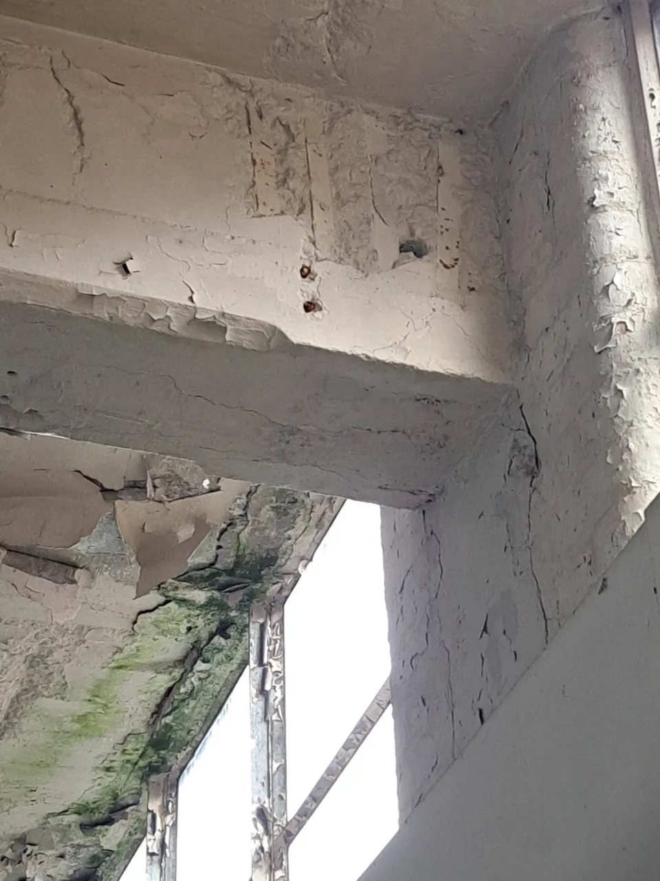
The field test, one photo at a time.

U-Net · ResNet-50 output on the same photo

InputU-Net · ResNet-50

Site photo

Model output

YOLO11x-segBest field recall (14 of 15 cracked images). Also flags some pipes and frames.U-Net · ResNet-50Cleanest crack morphology (mIoU 0.630). Suited to width and area measurement.FPN · EfficientNet-B418 defect classes at once. Each colour is a class from the DACL10k scheme.U-Net binary maskThe pixel map that downstream measurement works from.

What to look for

Beam soffit by a window

YOLO11x-seg marks the window mullions; U-Net keeps to the crack on the beam.

Real outputs from the dissertation's external validation on industry site photographs (Belfast). Drag the divider or use the slider to compare with the untouched input.

Chapter 04

Technical result

U-Net gave the cleanest crack boundaries (mIoU 0.630, precision 0.762, recall 0.787). It is the right choice when crack width and area must be measured.
On site imagery YOLO11x-seg was the most robust detector: it caught 14 of 15 cracked images and correctly cleared 13 crack-free images, where YOLOv8x-seg cleared only 1.
The 18-class model extended coverage to rust, spalling, drainage and equipment, which reduces false crack alarms. Thin classes remained weak, and I documented the reasons.
The integrated pipeline processed 689 industry images in 27 min 22 s. The same survey put a medium-sized building's manual inspection at 4–7 days.

YOLO-seg on the Crack-Seg test split

Box vs mask mAP50. Box localisation is strong; pixel masks are harder.

Box mAP50
Mask mAP50

View data table

Category	Box mAP50	Mask mAP50
YOLOv8x-seg	0.807	0.674
YOLO11x-seg	0.804	0.639
YOLO11n-seg	0.792	0.658

Source: MSc dissertation (Ulster University, 2025), Table 6

Field validation on 44 real site photos

Image-level results after manual verification (15 cracked, 29 crack-free).

Recall
Precision
Accuracy

YOLOv8x-seg matched YOLO11x-seg on recall but flagged 28 of 29 crack-free images, mostly pipes, shadows and coatings.

View data table

Category	Recall	Precision	Accuracy
YOLO11x-seg	0.93	0.47	0.61
YOLO11n-seg	0.67	0.33	0.43
YOLOv8x-seg	0.93	0.33	0.34

Source: MSc dissertation (Ulster University, 2025), Table 7

DACL10k per-class IoU: this study vs published benchmark

FPN–EfficientNet-B4 at 384 px, no auxiliary head (mIoU 0.317 vs 0.414 benchmark best).

This study
Flotzinger et al. (2023)

Thin, low-pixel classes (crack is ~0.3% of pixels) suffered most at reduced resolution. The dissertation reports this gap openly.

View data table

Category	This study	Flotzinger et al. (2023)
PEquipment	0.59	0.68
Graffiti	0.57	0.59
Hollowareas	0.55	0.54
Bearing	0.47	0.68
Drainage	0.47	0.52
EJoint	0.46	0.47
Rust	0.36	0.41
Weathering	0.36	0.42
ACrack	0.35	0.47
Spalling	0.29	0.37
Efflorescence	0.25	0.34
JTape	0.24	0.36
Wetspot	0.21	0.23
Restformwork	0.20	0.34
ExposedRebars	0.17	0.39
Rockpocket	0.10	0.27
Crack	0.07	0.29

Source: MSc dissertation evaluation outputs (per-class metrics)

Throughput per configuration

Seconds per image on an RTX 4060 (lower is faster).

View data table

Category	s / image
Crack U-Net	0.53
Crack-only YOLO	0.77
Multi-class segmentation	2.04
Full classification + report	2.38

Source: MSc dissertation (Ulster University, 2025), Table 8

Limitations, stated plainly

The multi-class model underperformed the published benchmark (0.317 vs 0.414 mIoU). Likely causes: 384 px inputs on an 8 GB GPU, no auxiliary classification head, and limited tuning.
The field set is small (44 images). It is a robustness check, not a statistically powered benchmark.

Outputs & artefacts

Site images where shadows and pipes were wrongly flagged as cracks — Fig. 01Failure analysis: shadows from steel members and hanging cables flagged as cracks.

Industry site photos with multi-class defect masks in several colours — Fig. 02Multi-defect predictions on industry inspection images (Fig. 19).

Multi-colour defect masks over site images — Fig. 03FPN–EfficientNet-B4 multi-defect predictions on industry imagery.

Grid of concrete crack tiles with blue predicted boxes and masks — Fig. 04YOLO11x-seg validation batch on Crack-Seg.

U-Net training and validation loss curves over 50 epochs — Fig. 05U-Net training and validation loss: fast convergence with a small generalisation gap.

Chapter 05

Practical impact & relevance

Shows how to choose a model by where it will be deployed. Benchmark mAP alone would have picked the wrong detector for site use.
Pairs a fast detector with a precise segmenter and a broad multi-class model. This is the architecture later taken forward in the AECAI product.

EvidenceWhere every figure on this page comes from

Each metric is taken from a primary record, not from a CV. Hover a metric to see its source. The underlying files are available for review at interview.

MSc dissertation (Ulster University, 2025)
MSc dissertation evaluation outputs (per-class metrics)
MSc dissertation figures
Ulster University MSc transcript (BLD811: 74)

Site photographs were supplied by Amphora Consulting for this research and appear in the submitted dissertation.

Next case study

AECAI: from inspection models to a working product